

How to work with Log Linear Models


An approach to applying log linear models (Generalized Linear Models) on categorical data with applications in ecological studies.
As data science practitioners, we arm ourselves with standard tools in our belt which we tend to put to use when we frame the problem domain to be one of classification or regression problem(for supervised learning), or a clustering problem (for unsupervised learning). These tools give a pretty good mileage for getting results on implementing machine learning solutions when applied to structured data.
In this article, I discuss a robust modeling tool to work with categorical data: Generalized Linear Model (GLM).
GLMs are widely used in social sciences, market research, health sciences where categorical scales are predominantly used. In financial services, insurance industry also use GLMs extensively. In market research, for example, a customer preference study done by a market research company on their customer panel between choice of a brand for a shampoo might ask them to state their choice between those made by L’Oreal, P&G and Unilever. The modeling here is used for identifying how to explain a customer’s choice or preference based on other variables (aka covariates), each of which is represented further in categorical scales.
What is categorical data?
Consider the following examples —
Ordered categorical data: A customer service survey showing customer respondes rating the service across choices {poor, ok, excellent}. There is a definite order from low to high in this list of categories.
Unordered categorical data: In a consumer preference study, a demographic variable of where the consumer lives could be a variable. Options may include {urban, suburban, rural.. etc}. There is no concept of order for this option.
GLMs are great tools to work with when working with studies that require analysis and modeling based on this type of data.
What is a Generalized Linear Model?
Before we get into the how, let’s briefly look at what GLMs are.
GLMs are a broad set of models that includes linear regression and ANOVA models for continuous data as response variables, as well as models for discrete responses. One such specialized cases of a discrete response model, for binary response is logistic regression model. This modeling technique is used for credit and other risk modeling in financial services as its known for its effectiveness, simplicity and parsimony as it applies to this domain. GLMs also allow for modeling a count (frequency) based response variable.
A GLM is made of three components —
1. A random component (Y) wherein we assume there is a certain probabilistic distribution.
2. A systematic component which represents the covariates or explanatory variables for the model.
3. A link function which represents the function of the expected value of Y. And this function allows Y to be expressed as some linear combination of the explanatory variables.
Modeling and Analysis with GLM
Next, let’s look at the analysis and modeling using GLM, along with code.
In this analysis we use a small dataset from the field of ecology where the day time habitat information of two lizard species — Grahami and Opalinus were collected. This data was obtained by observing specific information about habitat locations and the time when it was observed (McCullagh and Nelder, 1989).
Let’s look at the data to make sure we understand what an entire dataset of cateogorical data type looks like.
Lizard Species (L): Grahami or Opalinus indicating which species was observed. This is our target variable.
Illumination (I): indicating whether it was Sun or Shade.
Perch diameter (D): in inches with following values (aka factors): D≤ 2 and D> 2.
Perch height(H): in inches (H) with following values: H<5 and H≥ 5.
Time of day (T): also factor variable with three levels: Early, Mid-day and Late.
As we can see there are no continuous data, all of them are categorical data.
This modeling was implemented in R. You can implement this in your favorite language including Python. The concept of how to apply categorical data analysis and modeling is the same.
Let’s look at the data:
> lizard.data <-read.table(file = "lizard_data.txt",header = TRUE)
> head(lizard.data)
  Illumination Diameter Height   Time  Species Count
1          Sun      <=2    <=5  Early  Grahami    20
2          Sun      <=2    <=5  Early Opalinus     2
3          Sun      <=2    <=5 Midday  Grahami     8
4          Sun      <=2    <=5 Midday Opalinus     1
5          Sun      <=2    <=5   Late  Grahami     4
6          Sun      <=2    <=5   Late Opalinus     4
The data is setup in the form of what is called a higher order contingency table. We apply different log linear models on this data. We calculate the effect size, perform best model selection based on AIC. We also perform goodness of fit tests and residual analysis to assess model adequacy.
The steps taken for this analysis, output and discussion on the model performance are detailed below.
Fit log-linear models
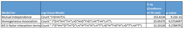
Using the lizard data, we first fit three log-linear models including:
(i) Model of mutual independence,
(ii) Model of homogeneous association,
(iii) Model containing all the three-factor interaction terms.
# Create the features from the dataset
I<-factor(lizard.data[,1])
D<-factor(lizard.data[,2])
H<-factor(lizard.data[,3])
T<-factor(lizard.data[,4])
L<-factor(lizard.data[,5])
Count<-factor(lizard.data[,6])
library(MASS) #need this package for using loglm
##create the three models first
#create saturated model
liz.model.sat <- glm(Count ~ I*D*H*T*L, family = poisson, data=lizard.data)
liz.model.sat$formula
#mutual independence
liz.model.mi <- glm(Count ~I+D+H+T+L, family = poisson, data=lizard.data)
summary(liz.model.mi)
#homogeneous association
liz.model.ha <-glm(Count ~ I*D+I*H+I*T+I*L+D*H+D*T+D*L+H*T+H*L+T*L,
family = poisson, data=lizard.data)
summary(liz.model.ha)
## then, get LRT stat (deviance, or, g-sq), aic, pearson x-sq, p-value for model
#mutual independence:
deviance(liz.model.mi) #152.6136
df.residual(liz.model.mi) # 41
AIC(liz.model.mi) #329.8624
mi.1 <- loglm(Count ~ I + D + H + T + L, data = lizard.data)
x2.mi<-mi.1$pearson
x2.mi #pearson chi sq is 157.8766
anova(liz.model.mi, liz.model.sat, test = "Chisq")
#p-value is 9.186e-15 ***
#homogenous association
deviance(liz.model.ha)#5.05375
df.residual(liz.model.ha) # 27
AIC(liz.model.ha) #230.3026
ha.1 <- loglm( Count ~ I * D + I * H + I * T + I * L + D * H +
D * T + D * L + H * T + H * L + T * L, family = poisson,
data = lizard.data)
x2.ha<-ha.1$pearson
x2.ha #pearson chi sq is 20.93927We then calculate the goodness of fit using residual deviance, which is the same as the G squared statistic (Goodness of fit), shown in Table 1 below.
Using AIC to determine best model
In order to get the goodness of fit, we need a saturated model, a model with df = 0. Unlike (binomial) logistic regression, we cannot solely use AIC because of possible conditional association between two or more terms in a log linear model. We begin the assesment by looking at model selection statistics including goodness of fit (LRT statistic, or deviance), p-value, AIC, Pearson Chi-squared value, and residual degrees of freedom.
Adding more complexity to the modeling
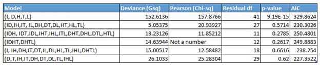
We evaluate the three models created in the previous section that is, single-factor terms, two-factor terms, and, all three-factor terms, and additionally setup a four-factor term based model (code below). Looking at rows 1 to 4 (Table 2), the mutual independence model fits very poorly.
## create a three factor interaction model, and get diagnostics

liz.model.trif <-glm(Count ~
                       I*D*H+I*D*T+I*D*L+I*H*T+I*H*L+I*T*L+D*H*T+D*H*L+D*T*L+H*T*L,
                     family = poisson, data=lizard.data)
summary(liz.model.trif)
deviance(liz.model.trif)#13.23126
df.residual(liz.model.trif) # 11
AIC(liz.model.trif) #250.4801
trif.1 <- loglm( Count ~ I * D * H + I * D * T + I * D * L + I *
                   H * T + I * H * L + I * T * L + D * H * T + D * H * L + D *
                   T * L + H * T * L, family = poisson,
                 data = lizard.data)
x2.trif<-trif.1$pearson
x2.trif  #pearson chi sq is 11.85212

anova(liz.model.trif, liz.model.sat, test = "Chisq")
#p-value is 0.2785
#create four factor interaction model
liz.model.fourf <- glm(Count ~ I*D*H*T+D*H*T*L,family = poisson, data=lizard.data)
# #Illumination*Species*Height*Time possibly has a zero in cross-class tab, so term removed
summary(liz.model.fourf)
deviance(liz.model.fourf) # 14.63944
df.residual(liz.model.fourf) # 12
AIC(liz.model.fourf) # 249.8883
fourf.1 <- loglm( Count ~ I * D * H * T + D * H * T * L, family = poisson,
data = lizard.data)
x2.fourf<-fourf.1$pearson
x2.fourf #pearson chi sq is NaN.
anova(liz.model.fourf, liz.model.sat, test = "Chisq")
#p-value is 0.2617Pruning too much complexity: Using StepAIC to evaluate
We need a model that is more complex than the homogeneous association model, but simpler than the three-factor and four-factor interaction term models. In order to get that, we then used StepAIC function by starting with the four-factor to evaluate models with different AIC, We also did the same step with three-factor term model. We picked the models in both cases with lowest AIC in either of them, and then proceeded to remove the redundant terms in each (picking models shown in Rows 5 and 6 in Table 2).
Based on this observation, we select row 6 (D,T,IH,IT,DH,DT,DL,TL,IHL) as the best model.
## setup multiple models, evaluate each using AIC and goodness of fit
#use stepAIC to manually select few models that 'appear' good for evaluation.

stepAIC(liz.model.mi) #329.9, residual dev = 152.6
stepAIC(liz.model.ha) #225.7, residual dev = 28.44,
stepAIC(liz.model.trif)#AIC: 227.4, residual dev =26.1.
stepAIC(liz.model.fourf)#AIC: 249.9, residual dev=14.64
##pick the lowest residual models and remove redundant params to fit few models
##and choose one final best model
#model 1
liz.model.besteval.1 <- glm(formula = Count ~ I + I:H + D:H + I:T + D:T +
+ D:L + T:L + I:H:L+ D:H:T:L, family = poisson, data = lizard.data)
#I:D:H:T + (fails to converge...so, term removed)
aic1<-AIC(liz.model.besteval.1)
aic1 #238.254
d1<-deviance(liz.model.besteval.1)
d1 # 15.00517
df.residual(liz.model.besteval.1) #18
anova(liz.model.besteval.1, liz.model.sat, test = "Chisq") #0.6616
besteval11 <- loglm(Count ~ I + I:H + D:H + I:T + D:T +
I:L + D:L + H:L + T:L + I:H:L + D:H:T:L, family = poisson, data = lizard.data)
x2.bestevall11 <-besteval11$pearson
x2.bestevall11 #12.58482
#model 2
liz.model.besteval.2 <- glm(formula = Count ~ D + T + I:H + D:H + I:T + D:T +
D:L + T:L + I:H:L, family = poisson, data = lizard.data)
aic2<-AIC(liz.model.besteval.2)
aic2 #227.3522
d2<-deviance(liz.model.besteval.2) #26.1033
d2
df.residual(liz.model.besteval.2) #29
anova(liz.model.besteval.2, liz.model.sat, test = "Chisq")#p-value is 0.62
besteval21 <- loglm(Count ~ D + T + I:H + D:H + I:T + D:T +
+ D:L + T:L + I:H:L, family = poisson, data = lizard.data)
x2.bestevall21 <-besteval21$pearson
x2.bestevall21#25.28304
liz.best=liz.model.besteval.2 #best model.
deviance(liz.best)Residual analysis of best model
Statistics for goodness of fit calculated above show a model that appears to fit to the data reasonably well. It is important that residuals are evaluated at each cell to show the quality of fit. Residual analysis can show that some cells may display lack of fit in a model that otherwise may appear to fit to the data well. We calculate standardized residual using rstandard function, where the observed and fitted counts are divided by their standard errors shown in Table 3 below.
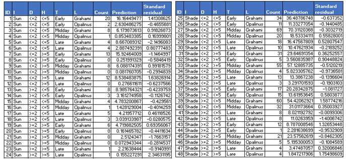
Table 3 output was generated using the following code:
#get residuals for best model
pred.best<-fitted(liz.best)
infl<-influence.measures(liz.best) #residual diagnostics
influencePlot(liz.best)
influenceIndexPlot(liz.best)
std.resid<-rstandard(liz.best, type = "pearson") # standardized resid
likeli.resid<-rstudent(liz.best, type = "pearson") #likelihood resid
liz.resid<-data.frame(I,D,H,T,L,Count, pred.best, std.resid, likeli.resid)
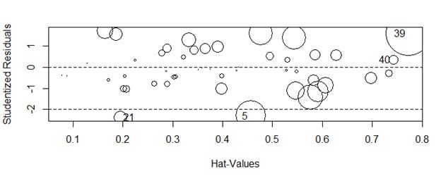
write.csv(file="lizard_residuals_pearson.csv", liz.resid)We perform several checks on the model including influencePlot. Figure below shows a few observations as outliers. A studentized residual value greater than equal to 2 or less than or equal to -2 is considered an outlier. We see two cells, a total of 5 count of lizards as outlier. The size of the bubble indicates measure of the influence of the observation, (it is the square root of cook’s distance).
Framing this as a logistic regression problem
We can also do a logistic regression where it would require us to transform the 48 record dataset to a 564 record dataset where each record represents the Grahami or the Opalinus species. That would allow us to predict for the given I,D,H,T condtions what lizard species might we find. In order to pursue this method, we convert lizard as response variable.
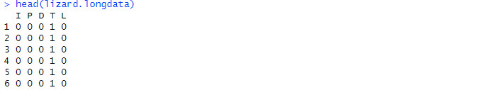
Data was converted to a long table with 564 observations, and each variable was recoded 0,1 for all variables and 1,2,3 for T. The header records looks like this:
library(car) # for using Anova
lizard.longdata <-read.csv("lizard_final_binomial.csv")
lizard.longdata
head(lizard.longdata)
lizard.longdata$L
liz.logistic <- glm(lizard.longdata$L ~ ., family = binomial, data=lizard.longdata)
#effects
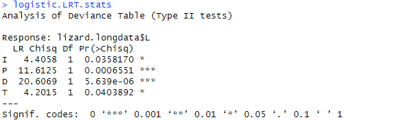
logistic.LRT.stats<-Anova(liz.logistic) #default test.stat is LRT, LRT stats
logistic.LRT.stats
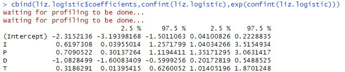
cbind(liz.logistic$coefficients,confint(liz.logistic),exp(confint(liz.logistic)))
anova(liz.logistic)
AIC(liz.logistic)
liz.logistic.sat <-glm(lizard.longdata$L ~ I*P*D*T, family = binomial, data=lizard.longdata)
We use Anova function from the car package to get the LRT stats which is shown below
The effects are shown in the table below for 95% confidence interval. The last two column show exponentiated CI.
Best subset using AIC
We applied stepAIC function on the full variable model which resulted in giving us the same model. In other words, it was the one with the lowest AIC value of 577.62, and a residual deviance of 567.6216.
L ~ I + P + D + T
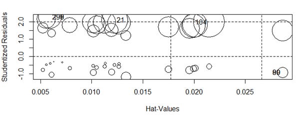
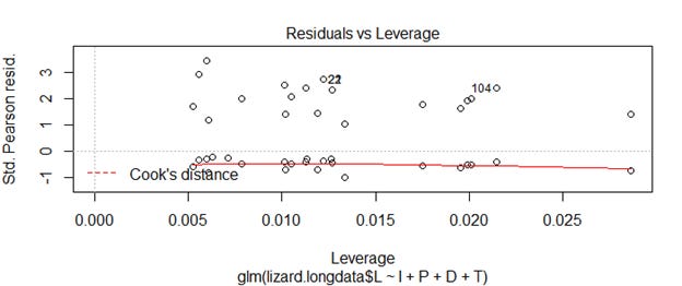
As we see in the influence plot below the residuals on the best model obtained is much higher than what we get on the loglinear model (Above influence plot for loglinear model).
We infer that this model does not fit the data well.
Final words on Logistic and Log-Linear model equivalency
It would make sense that the two models would be equivalent, we also know that the logistic model doesn’t know interaction terms. However, in this analysis we don’t see an equivalency, as the deviance of the two models are quite different. We have obtained 26.1033 for the best log linear model, and deviance of 555.4047 for the best logistic regression model.
We conclude a log linear model expresses the relationship nicely between the species and its variables that help us discern it.
There are a lot of great topics to delve into when working with categorical data. I will cover them in future posts. I hope this analysis was helpful in understanding how to work with GLMs.
Until next time!
References:
McCullagh, P., Nelder, J.A., 1989. Generalized linear models. London, Chapman & Hall, 511 p.
Agresti, A. 2007. An introduction to categorical data analysis. Wiley.
https://stats.stackexchange.com/questions/26930/residuals-for-logistic-regression-and-cooks-distance