

Multivariate time series forecasting and analysis of the US unemployment rate — Part 3

Multivariate time series forecasting and analysis of the US unemployment rate — Part 3

In my previous posts on this topic we covered two parts so far.
In Part 1, we discussed the importance and relevance of US unemployment rate forecasting and why a multivariate modeling approach is necessary.
We also discussed the various macroeconomic variables used in this analysis as well as an overview of the time series modeling approach.
In Part 2, we discussed the data prep steps as well as exploratory data analysis as it applies to standard time series datasets including time series decomposition, autocorrelation, partial autocorrelations as well as test for stationarity.
In this post, we will begin the discussion with step 5 of the 6 stepped process we outlined in part 1 of this series.
Let’s go to step 5:
5. Choosing and Fitting Models: In this step, models are trained using the training data and evaluated using validation data. These are chosen based on assumptions the researchers make that the model satisfies. Models are built using multiple parameter (or, hyperparameter values) to build the most efficacious model using historical data. In this post we will discuss Vector Autoregressive model as well as two Neural Network architectures.
Vector Autoregression (VAR) Models
A vector autoregression (VAR) model is a flexible time series model that is used for multivariate analysis. It is an extension of the univariate Auto regressive (AR) model and works with multivariate time series.
A VAR model contains a system of equations of n distinct, stationary response variables as linear functions of lagged responses and other terms. VAR models are also characterized p lags of all variables in the system, denoted as a VAR(p) model.
A bivariate VAR(2) model with time series variables y1t and y2t can be represented as follows:
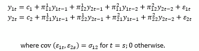
VAR models belong to a class of multivariate linear time series models called vector autoregression moving average (VARMA) models.
Interpretation of a general VAR(p) model is difficult due to complex interactions between the variables in the model. So the model is described using different types of structural analysis summaries including Granger causality, Impulse response functions and forecast error variance decomposition. This analysis includes Granger causality of other predictor time series data on the unemployment data. Granger causality is covered in part 4 of this series.
Whu use Vector Autoregressive Models?
VAR models are linear models. However, non-linearities can be modeled by applying various adjustments including number of lags to include for each time series, which co-variate to use, incorporating moving-average components and accommodating co-integration (Hyndman & Athanasopoulos, 2021).
The number of lags that are appropriate for forecasting the dependent variable is obtained by minimizing information criterion measures such as Akaike Information Criterion (AIC), Bayes Information Criterion (BIC), Hannan-Quinn Information Criterion (HQIC) and Final Prediction Error (FPE) (Lower, Eric, 2021). The lag that had the smallest information criterion value across all of these measures was chosen to provide a parsimonious model (ResearchGate, 2022). Deciding what variables to use can be done by applying Granger Causality tests. Granger Causality only provides the correlation across the variables and is not a true test of causality. In this analysis, the number of variables used for forecasting is small, so all the variables that were sourced were used for forecasting with VAR. Vector Autoregressive models have been proven to be useful for describing and forecasting economic and financial time series data. Similar to DSGE described above, VAR models are also used for structural inference and policy analysis (Zivot & Wang, 2003).
Artificial Neural Networks
The fundamental pattern based on which deep learning models are built is a perceptron. A perceptron has three set of nodes — (1) input nodes, (2) computational nodes, and (3) output nodes. Each set is called a layer. What uniquely differentiates a perceptron is that it has a single computational layer. This computational layer is also called the hidden layer.
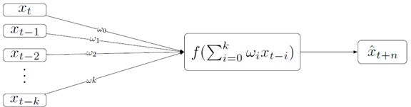
The perceptron model uses a linear combination of inputs with some weights. It then applies an activation function to produce an estimated output. This model takes input of k lags of time series x. And it estimates the value of the time series at a period t+n. The values ωo to ωk are the weights associated with each of the inputs. These weights are calculated using a cost function that minimizes the error, MSE (mean squared error). The perceptron without the activation function is nothing but a linear regression of the inputs with the weights. It is the transformation applied by the activation function that allows non-linearity of the underlying relationship to be modeled.
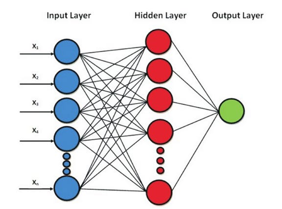
When there is one or more than one hidden layers wherein the information flows from previous layer to the next layer, the architecture is called Multilayered Feed Forward Neural Network.
The weights is what is used to determine which signal, or input should pass through. The weights are assigned randomly initially. An activation function (sigmoid, tangent hyperbolic (tanh), rectified linear unit (relu), or softmax) is applied to the linear combination of the input nodes. The result is passed to next layers, this step is repeated until the output layer which generates a vector of probabilities for various outputs. The resulting prediction is compared with actual values to determine error and this “feedback” is backpropagated to the nodes to readjust the weights and reapply the activation all over again. This is re-iterated until the cost function or loss function is minimized.
Why use ANN?
For this specific problem, non-linear relationship is assumed to be exist between the predictors and the target variables. ANNs are known to be effective in modeling non-linear relationships. ANNs were also found to be significantly better in forecasting unemployment rates when compared to autoregressive models. This however holds true when there is sufficient data, and the neural networks have an appropriate architecture and are not simplistic such as having a single hidden layer. In this analysis the neural network has a dense hidden layer. Further, the data obtained for this analysis is assumed to be sufficient to outperform autoregressive model. (Mulaudzi & Ajoodha, 2021)
Recurrent Neural Networks
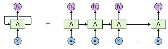
A recurrent neural network (RNN) is different from a plain vanilla neural network as discussed in the previous section in that a plain vanilla neural network accepts an input X that is of fixed length, and outputs a Y that is also of a fixed length. RNNs on the other hand can accept a sequence of inputs, more specifically, a sequence of vectors and output a sequence of vectors (Karpathy, 2015). In RNNs, the hidden layers store the information captured in previous stages of sequential data. The term ‘recurrent’ in RNNs is used because these neural networks perform the same task for every element of the sequence, specifically that of utilizing previously seen sequence to predict future unseen sequential data.
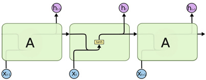
In Figure 3 below, the right hand side shows X at time 0 to time t. Each neuron or group of neurons, A produces a cell state h that is passed on to the next set of neurons. The cell state of the neuron at time t is remembered as ht. The left hand side shows the recurrence relationship of the pattern where h is updated at each time step. The right hand side shows the recurrence relationship in an unrolled view.
For an excellent reading on RNNs and LSTM, I recommend seeing Colah’s blog. Link to the original article is in references section.
Back to the discussion — The RNN can be represented mathematically in two steps occurring repeatedly across each time step. In the forward pass the following steps are done.
a. Calculate the hidden state: This is obtained by applying an activation function to the current input and previous state. The hidden state is given by
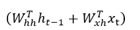
The tanh function applies a non-linearity and pushes the activation output to be in the range from -1 to +1.
b. Calculate the output: The output for time step t, formally y-hat of t, is obtained by
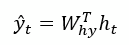
The learning that occurs in the RNN is really the calculation of the optimal weights across the three matrices that minimize the loss function. The matrices, again are:

Problem with RNNs
However, there is a drawback with a typical generic RNN that these networks remember only a few earlier steps in the sequence and thus are not suitable to memorizing longer sequences of data. RNNs when trained using backpropagation suffer from the vanishing gradient problem, wherein the gradients become so small that there is no real learning that can occur from inputs that were provided in the distant past time step. A class of RNN Long Short-Term Memory (LSTM) recurrent network overcomes this challenge.
LSTM is a special kind of RNNs that are designed to memorize long-term dependency in a sequence of data. There are four layers within each cell of LSTM as shown in Figure 4 whereas each cell of RNN has only one layer as shown in Figure 5.
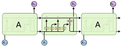
There are two types of information passing that occurs in LSTM. The top line shown in the cell in Figure 5 represents the information about the cell state. Information can be added to or removed from the cell state line which is controlled using gates.
The first layer uses a sigmoid activation to select between fully remembering or fully forgetting the information from the prior cell state. This is also called the forget gate.
The second layer also uses a sigmoid activation (also called as input gate layer), is used to select which information should be updated. The third layer uses a hyperbolic tangent activation that creates a vector of new possible values, that can be added to the cell state.
The next step is to update the new cell state by combining operations to forget what was determined to be forgotten and add new candidate value. The final step is to output which is based on a combination of sigmoid and tanh activations. The sigmoid activation determines which part of the cell state to output (sigmoid chooses between 0 and 1), whereas the tanh activation will finally push the output (tanh chooses between +1 and -1)
Why use LSTM?
LSTMs are essentially NNs that incorporate feedback loops. The architecture of LSTM described above allows for its use in sequence modeling. Specially, features of the data from the long running memory, as well as short term memory where most recent sequence of information is utilized. These models outperformed autoregressive models in an experiment conducted to forecast unemployment rates in the US (Mulaudzi & Ajoodha, 2021).
Next we’ll look at the setup for using the forecasting models and evaluating it.
6. Using and Evaluating a Forecasting Model:
The last step is to make forecasts and evaluate the performance of those forecasts. The model evaluation is performed to determine the efficacy of the models. In this analysis, back-testing is done with historical data.
Each of the neural network based multivariate model is compared with its corresponding univariate model. The multivariate models are also compared against one another. Finally, each of the multivariate model is compared with the Survey of Professional Forecasters (SPF) benchmark model data provided by Federal Reserve (Cook & Hall, 2017)
In traditional data mining methods when working with data that is not time series, k-fold cross validation is used to systematically divide the samples into k groups, where each group (in the k groups) is iteratively held out for model validation. This works for datasets that are not temporal in nature (they have no time dependency), therefore, in those cases each observation is independent.
Time series data has a unique characteristic in that there is a temporal dependence of variables. Machine Learning techniques require setting up a time series data as a supervised data set. In addition, this requires the splitting of the data for training the model and evaluation to be done differently from traditional machine learning methods.
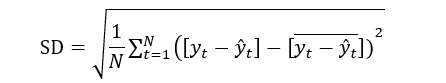
The models are compared against one another using the metric Mean Absolute Error (MAE) and standard deviation (SD). This is a well-known criterion for comparing forecasting accuracy of time series models. (Katris, 2019)
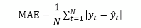
Where, yt is the actual unemployment rate for a period, and y-hat t is the forecasted unemployment rate for the same period, and N is the number of forecasts.
As this research is an extension of previous work done by researchers Cook and Hall (2017), this analysis uses the same feature UNRATE (unemployment rate data as made available by the Federal Reserve) for the same periods and partitioned the data for training and validation (1963 to 1996) as well as testing (1997 to 2014). The results obtained from this analysis were compared with the researchers results as well as other benchmarks referred to in the original paper. The creation of the validation data was done in the same manner as their paper by sequestering every 10th observation of the training data into a validation data set.
At this point we have all the elements ready for model building and evaluation. And that is what we will discuss in the next post.
References:
Colah’s blog: https://colah.github.io/posts/2015-08-Understanding-LSTMs/
Cook, T., & Hall, A. S. (2017). Macroeconomic Indicator Forecasting with Deep Neural Networks. Retrieved from dx.doi.org: https://dx.doi.org/10.18651/RWP2017-11
FRED. (2021–2022). Fed Reserve Economic Research. Retrieved from Fed Reserve Economic Data: https://fred.stlouisfed.org/
Hyndman, R., & Athanasopoulos, G. (2021). https://otexts.com/fpp3/. OTexts.
Karpathy, A. (2015). Retrieved from http://karpathy.github.io/2015/05/21/rnn-effectiveness/
Katris, C. (2019). Prediction of Unemployment Rates with Time Series and Machine Learning Techniques. Computational Economics, 682.
Lower, Eric. (2021). Introduction to the Fundamentals of Vector Autoregressive Models. Retrieved from Aptech: https://www.aptech.com/blog/introduction-to-the-fundamentals-of-vector-autoregressive-models/
Montgomery, A., & Zarnowitz, V. (1998). Forecasting the US Unemployment Rate. Journal of the American Statistical Association, 478.
Mulaudzi, R., & Ajoodha, R. (2021). Application of Deep Learning to Forecast the South African Unemployment Rate: A Multivariate Approach. IEEE Xplore.
ResearchGate. (2022). Retrieved from researchgate.net: https://www.researchgate.net/post/How-do-you-choose-the-optimal-laglength-in-a-time-series
Vector Autoregressions. (2022). Retrieved from Statsmodels: https://www.statsmodels.org/dev/vector_ar.html
Zivot, E., & Wang, J. (2003). Vector Autoregressive Models for Multivariate Time Series. In E. Zivot, & J. Wang, Modeling Financial Time Series with S-Plus®. New York, NY, USA: Springer. doi:https://doi.org/10.1007/978-0-387-21763-5_11