

Multivariate time series forecasting and analysis of the US unemployment rate — Part 4 (Final)

Multivariate time series forecasting and analysis of the US unemployment rate — Part 4 (Final)

In the final part of this series we will compare the results of our modeling work between classical time series models and neural network architectures applied with multivariate data that we previously discussed vs the univariate benchmark models.
If you haven’t read the previous posts, please do take a moment to review them. I have added a brief summary below outlining what was covered along with links to those articles.
In Part 1, we introduced the importance of US unemployment rate forecasting as well as how a multivariate modeling approach can be applied.
We also discussed the various macroeconomic variables used in this analysis as well as an overview of the time series modeling approach.
In Part 2, we discussed important data preparation considerations, as well as exploratory data analysis as it applies to standard time series datasets. We covered time series decomposition, autocorrelation, partial autocorrelations as well as ADF test for stationarity.
In Part 3, we discussed how Vector Autoregressive (VAR) models work. We also covered two neural network architectures including Artificial Neural Network and Recurrent Neural Networks and a discussion on LSTMs. We concluded the discussion in part 3 with model evaluation metrics used for this work.
Model development procedures
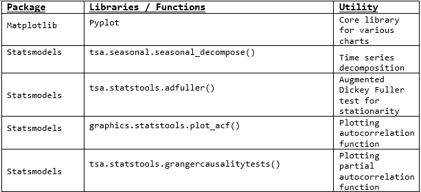
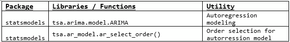
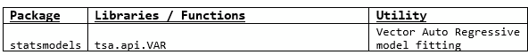
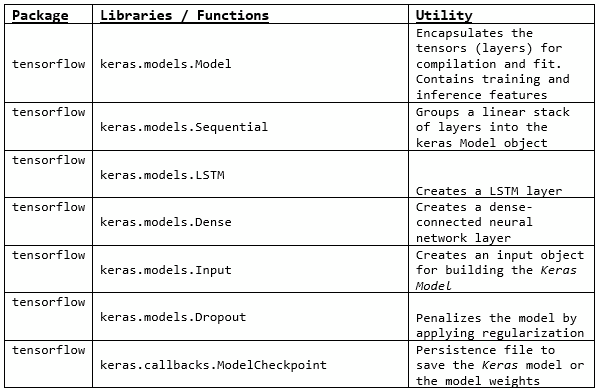
For forecasting the unemployment rate, each of the three methods are first used with a univariate setting, followed by multivariate model fitting and forecasting. The model development was done using Python libraries (version 3.8.5). The details on specific packages and functions are listed in the below tables:
Classical Time Series — Univariate analysis
An optimal lag order of 5 was used for univariate model fitting. It is obtained by fitting the model with a max lag of 24 when calling the ar_select_order() function using ‘aic’ as the information critieron. The model is fit using the ARIMA library from statsmodels package and a 12-step forecast is obtained. The summary() function provides the below results for AR(5):
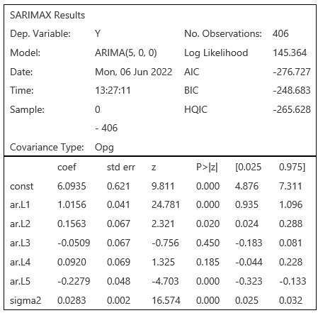
The model fit results are shown in above output for AR(5) model. Lags1, 2 and 5 are found to be statistically significant along with a white noise component sigma2.
Once the model is fit, walk forward multi-step forecasting for a forecast horizon of 12 is done. This is inclusive of all forecast horizons until 12. This forecast is done by providing end of the training period as starting period for forecasting, along with a lag of 5 as the input. Each forecast call returns a forecast for the next 12 periods. The input vector is changed by sliding the input window forward (walk-forward) by one incremental observation at a time and selecting the next 5 observations as input. Each output vector of the 12 forecasted values for the different forecast steps is separately stored in a list.
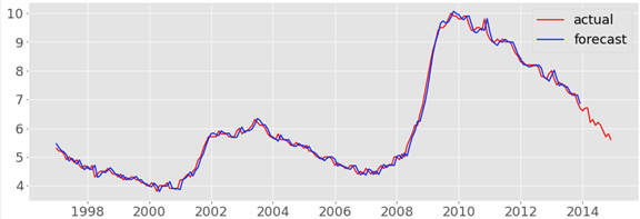
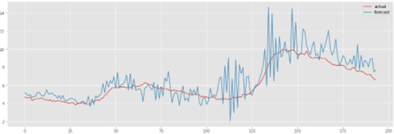
Mean Absolute Error is calculated by comparing the lists of actual unemployment rate for the various forecast horizon with the lists containing forecast value from above. Time series data for forecast and actuals is plotted as shown below in figure (forecast in blue, and actuals in red).
The validity of the data setup is tested by comparing the results of the AR model developed in this analysis for a single forecast horizon window and comparing it with results obtained in the Federal Reserve paper (Cook & Hall, 2017). The MAE obtained is 11.5 bps (basis points). Results of this test and others described in sections described further are summarized in the results and discussions section.
Classical Time Series — Multivariate analysis
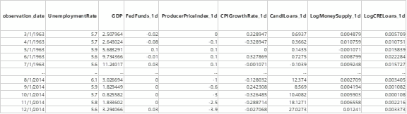
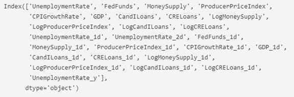
The standard VAR(p) model implementation from statsmodels is not appropriate for non-stationary data, so dataset in this analysis is made stationary. (Vector Autoregressions, 2022). The results of ADF test applied across the entire list of variables was discussed in part 2 of this series. The following variables that are shown (and only the leading and trailing records are displayed) in the full time series data, were used for fitting the VAR model.
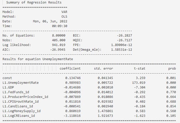
Again, max lags of 24 is provided to determine optimal lag, where BIC provides 1 as the optimal lag. For selecting the lag select_order() function from statsmodel package is used. Partial output has been reproduced below. The results show that the unemployment rate and the GDP at lag = 1 are statistically significant to explaining unemployment rate at current time t.
Granger causality
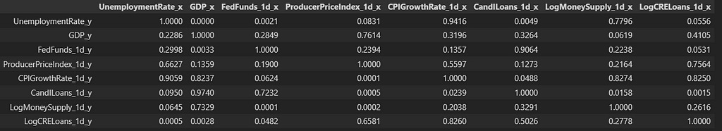
Granger causality test is done using grangercausalitytests function from statsmodels which provides the following results. We pass the value of 1 to maxlag parameter.
The tests indicate that consumer price index growth rate (CPIGrowthRate1d_x), and Money Supply (LogMoneySupply_1d_x) both are positively correlated with Unemployment Rate (UnemploymentRate_y) and granger causes Unemployment Rate. It is important to note that, though the name suggests “Causality” it is not meant to imply causality. The differentiating phrase used is variable x “granger causes” variable y. A better way of thinking about it is that it translates to correlation between the two variables.
The values in this table show the p-values, and, if they are less than the significance level (0.05) then it implies that the coefficients of the corresponding past values is zero, which is to say, the null hypothesis that X does not “granger” cause Y can be rejected.
Classical Time Series — Forecasting
Rolling forecast is applied to get multi step multi output for 12 step horizon using the forecast function from the fitted VAR model. The rolling forecast is obtained in the same way it was done for univariate analysis by creating separate lists to store the actual unemployment rate for various forecast horizons as well as for storing the forecasted unemployment rate fot those forecast horizons. The mean absolute error is then calculated across these lists for each forecast horizon consecutively and reported.
Following results are obtained by calling the mean_absolute_error() function from sklearn.metrics package. This is done by providing the list with forecasted values along with actual values, one list each for the 3,6,9 and 12 step forecast. The MAE were obtained as 11.2 bps, 19.7 bps, 27.7 bps and 35.9 bps respectively. (More summarized comparative views below).
Model development using Neural Networks
A key experimental setup that is replicated across all of the neural network architectures in this analysis across univariate and multivariate analysis is the process of setting up validation data set from the original training dataset, which is from 1963 to 1996. In this dataset, every tenth observation is removed from training data set and passed into a validation data set. Each observation is a set of continuous 36 month data. This dataset is then used to evaluate the performance of the trained model. The testing dataset contains the remainder of the monthly data from 1997 to 2014.
Since this analysis is meant to compare an existing univariate work in a new multivariate setting, we retained the experimental settings similar to univariate work by Cook and Hall. In their work, they use a lag of 36 months of the unemployment rate data for neural networks. Therefore, this analysis also uses lag of 36, specifically for the univariate analysis using ANN. Lastly, they also use the original unemployment rate, the first order difference and the second order difference unemployment rate in the univariate model. The setup for univariate forecasting in this analysis is replicated with their setup.
When working with Neural Networks it is important to standardize the data, particularly when the data is not scaled. If the data is not standardized, attributes that have higher values will take on higher weights in the model incorrectly influencing the model. For this analysis neural network models have been evaluated separately with both standard scaling and min-max scaling. The sklearn scaler object is fit with the training data separately for dependent and independent data. Then as the next step, independent data (x) is transformed. The scaler object is not fit with testing data so as to avoid data leakage.
As discussed in the data preparation section, there are two different types of data transformation applied: (1). Standardization and (2) Min-Max Normalization. Each neural network is trained, evaluated and used for forecasting. The final results are reported based on the best model evaluation metrics across the two types of transformation. When the model is trained, and forecast is generated, the forecast is reverse transformed to original scale of the data for calculating mean absolute error.
When working with machine learning algorithms including deep learning algorithms, time series problem needs to be converted into a supervised learning problem. This is done by taking sequences of data iteratively from the original time series and splitting the time series data into a set of time series data for training, and another set of time series data for testing. It is in this set of training sequences, the sequestering (hold out) operation described above is done for model evaluation.
For LSTM under univariate setting, the number of lags is chosen to be 12. On splitting the training data into training and valiation, X training data is obtained with the shape (344,12,3) with 344 samples, 12 lags, and 3 features. The Y training data is of the shape (344,12) with 344 samples and 12 lags. The testing dataset is setup in the same way without the need to sequester any observation, that provides a X testing data of the shape (194, 12, 3) and Y testing data of the shape (194, 12).
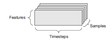
TensorFlow from the keras package in Python is used for implementing the neural network architectures in this analysis. A tensor is a 2D matrix with additional dimensions. A 3D tensor is an appropriate data structure to store time series data. This can include storing the samples, time steps and features, which is useful especially for a multivariate problem as shown in figure below.
Keras model development workflow:
The workflow required for model development using Keras requires is as follows (Chollet, 2018):
1. Define the training data using numpy arrays or tensors.
2. Define a model that is a network of layers which maps the inputs to outputs.
3. Choose a loss function, optimizer and a model evaluation metric for monitoring the model training
4. Loop through the training data by calling fit() method
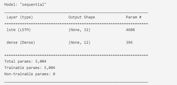
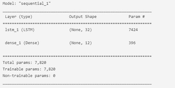
A Tensorflow model is defined by creating an object of the class Sequential() that creates linearly stacked layers. A LSTM layer is added with 32 nodes, relu activation function along with the specification of the input shape that includes the number of lags, and number of features. This is followed by addition of a Dense (final output) layer with as many nodes as the number of forecast steps. A ModelCheckpoint is created to save the best model information based on lowest validation loss. Finally, the model is compiled by choosing ‘adam’ optimizer and the model is set to be optimized for lowest MAE.
On fitting the LSTM model with 100 epochs, following summary results shows the type of layers is obtained. It shows the two linearly stacked layers LSTM and Dense.
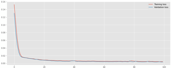
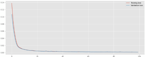
The training loss and validation loss drops in less than 10 epochs, and plateaus after 50 epochs as shown below.
A12-step horizon using the best model was obtained. Which was then then reverse scaled to calculate the error on forecasted data. Following results were obtained for univariate LSTM:
Overall mean absolute error in percent : 0.3539
Overall mean absolute error in basis points : 35.39
The below chart shows the forecasted vs actual value for the 0th step forecast (first month) in the 12 month forecast horizon.
Discussion on Multivariate forecasting with LSTM
The setup for multivariate forecasting for LSTM is the same as that for univariate except for the data setup. The supervised data set for training and testing includes multiple variables as shown below.
The tensors setup for multivariate forecasting are of the following shape
XTrain: (344,12,25)
YTrain: (344,12)
XTest: (194,12,25)
YTest: (194,12)
LSTM model for multivariate forecasting is also setup with two layers as shown below:
The training loss and validation loss are outputted as follows. The loss convergence is similar to the univariate LSTM model training.
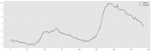
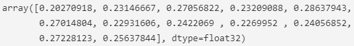
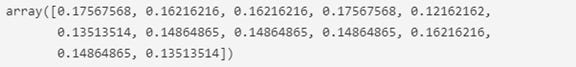
The model evaluation error obtained is 0.0292. Again, forecasting with the best LSTM multivariate model, a vector of 12 step forecast is obtained. For illustration the first record of the forecasted values and actual values are reproduced below:
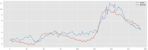
Compared to the univariate LSTM mode the forecast for the first month of the 12 month period shows lesser accuracy (as you will see, not good!). The chart below shows the performance of the LSTM multivariate model after inverse transforming the forecast.
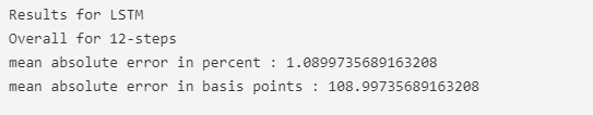
The MAE for the the 12 step forecast horizons is as shown below:
Discussion on Univariate Forecasting with Feed Forward ANN:
For fitting an ANN model using Tensorflow in Keras, the data used for LSTM needs to be reshaped such that the structure of the input data is stored as (samples, features). In this analysis, forecasting using ANNs was done with both min-max scaling and standardization scaling. The model results were better when using standardization for univariate setting, while the results were better when using min-max normalization for multivariate setting.
All the other experimental conditions were retained as before, an input lag of 12 was chosen. Again, two linearly stacked layers were chosen for fitting the ANN. The univariate model output was obtained as follows:
After fitting the model, MAE of validation was obtained as follows:
After fitting with the best model, forecasting the 12-step output, and inverse transforming, the following plot is obtained:
The MAE for the 12 step forecast with the univariate ANN is obtained as shown:
Discussion on Multivariate Feed Forward Artificial Neural Network
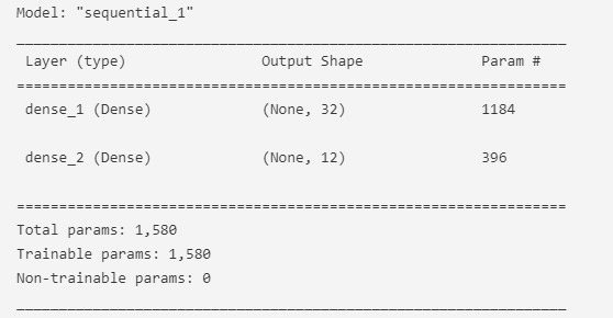
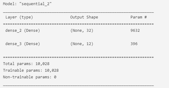
This model is also a 2-layer linearly stacked neural network. The model information is provided below.
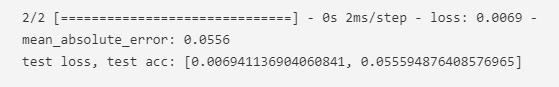
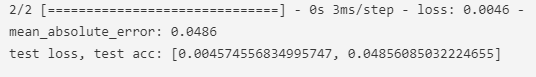
The test loss and test accuracy is shown as below:
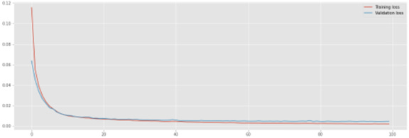
The training loss and validation loss is plotted below:
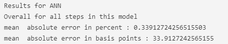
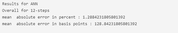
Again, after forecasting with the best model, inverse transform is done followed by calculation of the MAE. Results obtained are shown below.
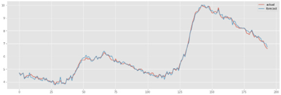
The plot for the first month forecast in the 12-month forecast horizon is plotted below.
Of all of the model used so far, it is easy to tell visually that this model performs poorly (of all the other models) developed in this analysis.
Let’s look at how we did across all the models.
Model Evaluation Results
A comparative analysis of the models is tabulated as shown in table below.
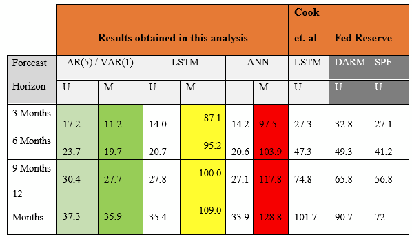
The Mean MAE is shown for the VAR, ANN and LSTM models. Each model has an univariate (U) and multivariate (M) result tested on out of sample data from 1997 to 2014.
The last column shows benchmarks obtained from the data published by SPF (Survey of Professional Forecasters) at Philadelphia Federal Reserve Bank. These benchmarks were used for comparison of univariate analysis and forecasting by Cook and Hall (2017). This analysis used the same data and benchmarks as the previous analysis by the Fed Reserve authors which was done using univariate methods.
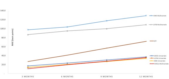
The below figure shows graphical assessment of the MAE of the different models over the multiple forecast windows when compared to the SPF benchmark. The brown line in the center indicates the SPF forecast. The top two lines indicate the multivariate neural networks. The bottom four lines indicates the univariate AR model, neural networks and the VAR(1) multivariate model. A comparative explanation of models generated from this analysis vis-a-vis the benchmarks follow.
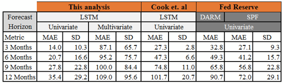
This research Univariate vs Fed Univariate — In this analysis, the AR(5) model compared relatively better than Fed’s Directed AR Model (DARM). It performed just marginally better than SPF’s forecast. It also performs better than benchmark univariate LSTM. While there is not enough information on the model specific hyper tuning parameters used in their univariate LSTM, it is plausible their model could perform equally well under similar parameters. It is also plausible that the univariate AR model from this analysis outperformed the directed AR model because of the usage of optimal lag and usage of first order and second order difference as model inputs. There is no information on how the DARM was setup by Federal Reserve to further comment on causes for performance differences between the two.
This research Multivariate VAR Model Performance — The VAR model from this analysis performed best for the three month forecast period, with comparable performance with the neural network univariate models for six month and nine month forecast period, while its performance was slightly unfavorable compared to the twelve month forecast period. The multivariate VAR(1) model outperformed the univariate AR model across all quarters with diminishing gap in their performance as the number of forecast steps increased. It also performed better than the vanilla LSTM model by Cook & Hall and other Federal Reserve models. Based on these results obtained in the VAR model, it can be concluded that the information contained in the macroeconomic indicators chosen for forecasting unemployment rate have a reasonably strong relationship with unemployment rate, more than the strength of the relationship solely found as a result of autocorrelation of lagged unemployment rate data, at least for shorter forecasting period.
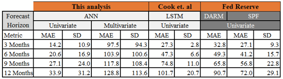
This research Univariate Neural Network models — The univariate ANN and LSTM models performed better than VAR(1) specifically for the 12 step forecast period with comparable performance for three and six step forecast periods. It is possible that a more optimally tuned neural network and other architectures might be able to beat the VAR(1) model not just for the longer step forecast periods, but consistently across all the periods.
This research Multivariate Neural Network models — The neural network models showed promisingly low MAE for validation data. However, both LSTM and ANN fared poorly on the test data. The LSTM model had two to three times the MAE on an average compared to SPF models. This is likely due to reasons such as overfitting and propagating errors due to predicting multiple variables.
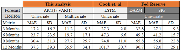
The three subsequent tables below show the MAE and Standard Deviation for each models developed in this analysis and they are compared with benchmark MAE and Standard Deviation. The standard deviation was computed for the forecast errors. Three of the models — multivariate VAR(1), univariate LSTM and univariate ANN have a smaller dispersion around the mean when compared to the dispersion of the SPF benchmark model around their respective means. Whereas, the univariate AR(5), multivariate LSTM and multivariate ANN all have a larger dispersion compared to that of the SPF benchmark models. All of models developed in this analysis, including the best performing multivariate VAR(1) model have a larger dispersion around the mean relative to Cook & Hall’s standard deviation around their model means. MAE and SD are in basis points.
Conclusion
One of the questions this research set out to answer was whether adding more variables helps improve model performance. The results established that is true, as shown by the results of the multivariate vector autoregressive model, specifically for shorter forecast windows.
Another question this research sought out to answer was whether using a neural network model can help improve the forecast accuracy. The results provide a mixed answer to this question. The univariate neural network models — both ANN and LSTM did favorably well when compared to Fed’s models. However when more data was introduced into the neural networks, the model performance deteriorated significantly. The neural networks had minimal tuning. It is possible that under the right set of hyper parameters, as well as by using other more recently developed neural network architectures may result in better outcomes for forecasting unemployment rate.
Limitations
One of the limitations of these models is they are not grounded in the economic theories that underpin the relationship between the macroeconomic variables. So, attributing causality from any of the other multivariate features to explain the dependent variable is not feasible. This research can be extended using Structural VAR which allows modeling assumptions of directional relationship between the various variables.
This research also did not consider implementation of cointegration in these models, which in finance and economics is the idea of equilibrium achieved between two different economic variables over a long run (Zivot & Wang, 2003).
Recommendations for further research
There are several avenues that can be explored in the future to extend this work.
There is an opportunity to expand the VAR model by including other variables that can explain unemployment rate, variables related to other economic activity such as stock market returns, private investments such as equity financing and many other economic indicators.
Explore other recurrent neural network architectures such as Bi-directional LSTM in a multivariate setting.
Employ permuting of multivariate combinations as well as hyper parameter optimization for neural network training.
There is volatility in the unemployment rate which could be modeled using Generalized Autoregressive Conditional Heteroskedasticity (GARCH) to handle different volatility across different times.
The unemployment rate appear to in different regimes across different long-run economic cycles. One option to model this would be to use regime switching using Hidden Markov Models (HMM).
Lastly, and importantly, with recent advancements in transformer architectures and its application to time series data, there is an opportunity to consider implementing these architectures to forecasting unemployment rate.
In closing, this was an interesting and very worthwhile exercise in applying academic rigor to real world financial forecasting application. This work was the basis of my talk at ASA (American Statistical Association) Symposium on Data Science and Statistics at Pittsburgh, PA (June ’22)
I know there are many other considerations I could have included in the analysis. I welcome your comments/feedback, and look forward to being in broader conversation with you on application of data science techniques.
Acknowledgement
A shout out and acknowledgement to all the researchers, educators and authors who spent countless hours building and teaching this knowledge base over the many decades. It is only out of their efforts do data science practioners like myself are able to do what we do. I am grateful to all of you.
Until next time!
References:
Chollet, F. (2018). Deep Learning with Python. NY: Manning.
Cook, T., & Hall, A. S. (2017). Macroeconomic Indicator Forecasting with Deep Neural Networks. Retrieved from dx.doi.org: https://dx.doi.org/10.18651/RWP2017-11
Karpathy, A. (2015). Retrieved from http://karpathy.github.io/2015/05/21/rnn-effectiveness/
Montgomery, A., & Zarnowitz, V. (1998). Forecasting the US Unemployment Rate. Journal of the American Statistical Association, 478.
SPF. (2022). Survey of Professional Forecasters. Retrieved from Federal Reserve Bank Philadephia: https://www.philadelphiafed.org/surveys-and-data/real-time-data-research/survey-of-professional-forecasters
Vector Autoregressions. (2022). Retrieved from Statsmodels: https://www.statsmodels.org/dev/vector_ar.html
Zivot, E., & Wang, J. (2003). Vector Autoregressive Models for Multivariate Time Series. In E. Zivot, & J. Wang, Modeling Financial Time Series with S-Plus®. New York, NY, USA: Springer. doi:https://doi.org/10.1007/978-0-387-21763-5_11