

Reverse sentiment based ranking classification from Amazon product reviews


This article describes how amazon reviews can be interpreted and classified back into a low or high rank using a bag of words vectorization approach to generate sentiment based on the comment or review left by the buyer.
We perform analysis of comments submitted by buyers of a specific product on Amazon.com and applying NLP techniques to the reviews combined with overall score (1 to 5) as provided by the buyer.
For the purpose of this analysis, a single product referenced by ASIN (Amazon Standard Identification Number), akin to SKU on a retail outlet floor was used. This product name as sold on Amazon is “AcuRite 00613 Digital Hygrometer & Indoor Thermometer Pre-Calibrated Humidity Gauge”.
At the time of this analysis, it retailed for less than $15, under product category of “Industrial & Scientific”. And, there were 21K ratings viewable on amazon.com. The dataset that is used from an archive obtained for this project has 1,229 reviews for this product specifically, along with the detailed text review as well as product rating.
The objective of this analyis is to predict what rating might the user provide based on the sentiment expressed in the comments. As Amazon ratings are on a 1 to 5 scale, for sake of simplicity, this 5-class problem was created as a 2-class problem by combining ratings {1,2,3} into “Low” rating, and, ratings {4,5} into “High” rating.
How natural language processing is applied in this analysis:
There are three main steps in this analysis.
(1) Data acquisition and pre-processing of the text data.
(2) Vectorizing the data using bag of words.
(3) Applying Naïve Bayes’ classifier on this vectorized text data to create a predictive model that takes a comment and predicts the user sentiment as Low or High.
A preview of model results
The classifier is highly accurate in predicting both “High” and “Low” ratings, with a F1-score of 0.96 & 0.97 for each class respectively. On inspecting the actual comments, we can see that the predictor did a good job of attributing sentiments such as “works really good”, “works as advertised”, “awesome addition” to a High rating, and attributing sentiments such as “why bother with reviews”, “way off”, “worked fine for a month, but” to a Low rating. Though you will see the way the model in this analysis actually works is not by inferring the sentiment based on sequence of words as described above in quotes, but rather on the count of words. M
We close this analysis with some limitations and improvements (and if you guessed Transformers as options — you are right!). So, let’s review:
Step 1: Data Acquisition and Preparation
The data used for this analysis is different from a standard “corpora” dataset in that the original data owned and tracked by Amazon.com is stored as a tabular data with 12 attributes. Of interest to this analysis are only few attributes that were retained. It includes the following:
· reviewText — The actual text comments entered by a buyer
· summaryStr — Summary of the comments as provied by the buyer
· overall — The original rating on a 1–5 scale.
· ASIN — This is the unique ID for a product as noted earlier.
The data used for this analysis was obtained from an archive on ucsd.edu domain. The original file is in JSON format and has 77,071 reviews.
As the original file obtained for the analysis had ratings and comments for a number of products under the category of “Industrial & Scientific”. We picked one specific ASIN (product) on which this analysis could be performed. A group by operation was performed using valuecounts() function to get count of records based on ASIN, and the one with the most records were used for this analysis. The rationale for choosing ASIN with highest number of records was so that we could work with a reasonably larger number of records to train and test the classifier. The finally processed dataset was of the shape 1229 x 4. The 4 members in the DataFrame are of “object” type, and therefore need to be typecasted into string (for review) and int (for rating) formats.
from urllib.request import urlopen
from nltk.corpus import stopwords
from sklearn.feature_extraction.text import CountVectorizer
from sklearn.feature_extraction.text import TfidfTransformer
from sklearn.naive_bayes import MultinomialNB
from sklearn.metrics import classification_report
from sklearn.model_selection import train_test_split
from sklearn.pipeline import Pipeline
from sklearn.metrics import confusion_matrix
import nltk
import os
import json
import gzip
import pandas as pd
import wget
import matplotlib.pyplot as plt
import seaborn as sns
import string
url="http://deepyeti.ucsd.edu/jianmo/amazon/categoryFilesSmall/Industrial_and_Scientific_5.json.gz"
textfile=wget.download(url)
data = []
with gzip.open(textfile) as f:
for l in f:
data.append(json.loads(l.strip()))
# total length of list, this number equals total number of products
print(len(data))
# first row of the list
print(data[0])
#quick review of data structures - list, df
df = pd.DataFrame.from_dict(data) #convert dictionary to dataframe
#check length of dataframe
print(len(df))
#check content of first record
df.iloc[0]
#check comments of first record
df.reviewText.iloc[0]
#check summary stats of the dataframe
df.asin.describe()
#alternative way to find the most frequently occuring ASIN to identify candidate product for analysis
df['asin'].value_counts() #shows B0013BKDO8 has the most ratings
asindf=df[df['asin']=='B0013BKDO8'] # keep product of interest
#check shape of new df
asindf.shape #reduced to a single ASIN as above.
asindf=asindf[['asin','overall','reviewText','summary']] # keep four colsBasic Exploratory Data Analysis
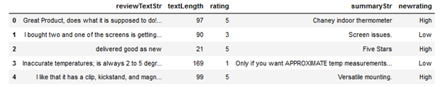
Here is a quick view of what this datset looks like. The last column called newrating was created by additional data processing described below.
There are only four variables originally retained, so EDA is quite quick to do. First, let’s see textLength.
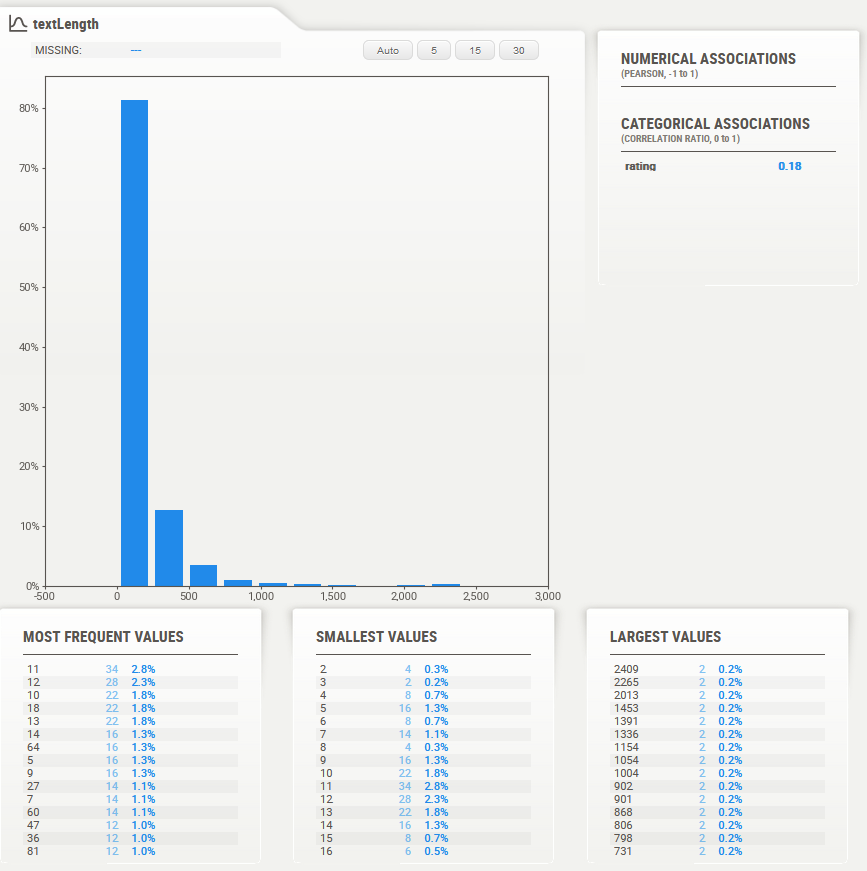
The above chart shows the distribution of the length of the text comments buyers provide in addition to their ratings. And this is what the distribution looks like. Average length of the string is 153 chars with a standard deviation of 239. This is a highly skewed distribution.
import klib as kl
kl.dist_plot(finaldf.textLength)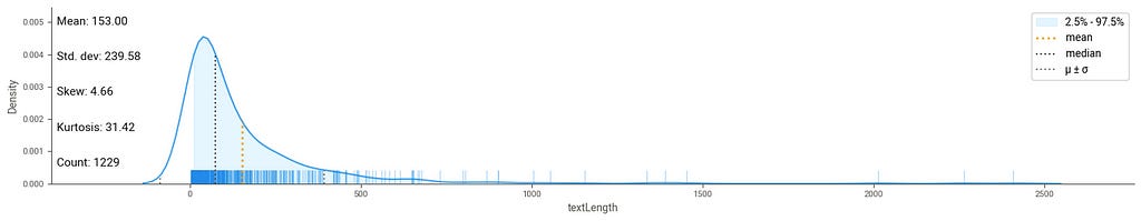
Interestingly, longer text is associated with higher ratings as seen in this box plot.
plt.figure(figsize=(15, 5))
sns.boxplot(data=finaldf, x="rating", y="textLength")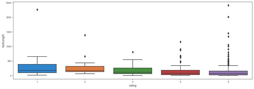
Next, we’ll see the rating.
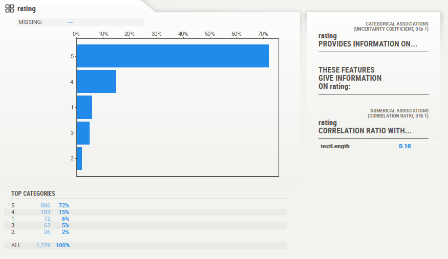
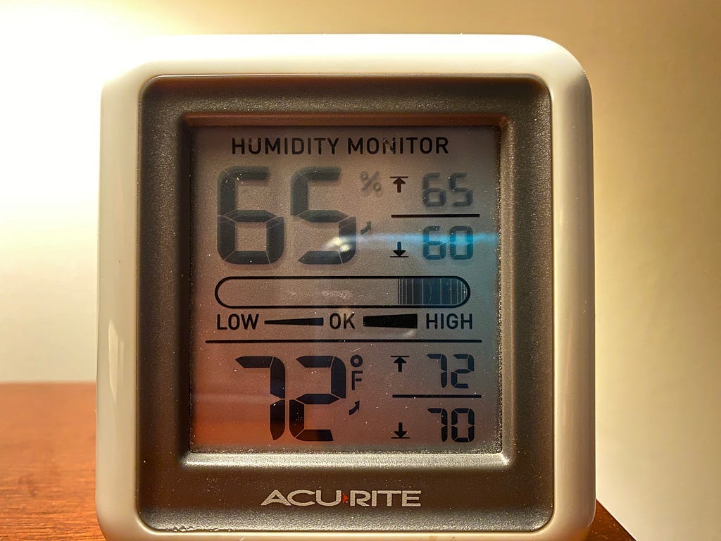
This is an interesting observation, ratings are heavily skewed towards 5, then followed by 4. This must be one of those really well performing products for most buyers. I certainly can vouch for that that because I own one of this, and it is always by my bedstand. Here is the picture of the device I bought many years ago (still working well!)
The correlation of text length to rating is very low (0.18). As we can also see beow there is hardly anything discernable about the impact of comment length to the 5 separate ratings.
We binarize the ratings with a new attribute called newrating, which has two values {Low, High}. Ratings 1,2,3 are binned under Low. Ratings 4,5 are binned under High.
# derive new rating
def set_new_rating (row):
   if row['rating'] == 1 :
      return 'Low'
   if row['rating'] == 2 :
      return 'Low'
   if row['rating'] ==3 :
      return 'Low'
   if row['rating'] ==4 :
      return 'High'
   return 'High'


finaldf['newrating'] = finaldf.apply(set_new_rating, axis=1)
Step 2: Text Pre-processing for natural language processing
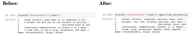
There are a few key elements that are being used for text preprocessing. We do the following steps:
a. removing punctuations by reading comments.
b. removing English stopwords.
c. returning a list of clean tokenized words.
The reviewText before and after this processing appears as shown below:
Following code block shows the text pre-processing:
from nltk.tokenize import word_tokenize


def text_processing(varText):
    review = [char for char in varText if char not in string.punctuation]
    review= ''.join(review)
    return [word for word in review.split() if word.lower() not in stopwords.words('english')]
For removing punctuation, each character is checked against the String.punctuation — a constant string that is a property of the string object with a value of ‘’!”#$%&\’()*+,-./:;<=>?@[\]^_`{|}~’
Where a match isn’t found, that character is retained and joined back into a string. Therefore, this string was split again to create words, to then compare against English stopwords imported from NLTK.corpus. Examples of stop words include words that are frequently used in English which typically don’t carry weight in most text analysis such as “I”, “me”, “myself”, “we”, etc. Each reviewText was processed to generate tokens in this manner
We could have also applied stemming and lemmatization (tokenizing similar words down to a single word e.g. did, doing, done are treated as the same word). This allows similar words to be tagged as the same word allowing for a more precise weight calculation of the presence of such words. It was left out in this exercise, however.
Vectorization
Each review is converted as a list of tokens. Each review is now converted as a vector to train the classifier model. We apply bag of words (bow) model to this text. We use Scikit Learn’s CountVectorizer to convert word in each of the comments into a matrix of token counts (not the token itself — since, we already achieved that in the previous step). This allows creating a vocabulary of 2,326 words in the dataset and counts occurrence of each word. This same step is applied to individual comments to create a matrix of 1,229 records X 2,326 words. We get a sparse matrix of this dimension with a sparsity index of 0.57%.
An individual record is profiled here for illustration. The 8th reviewers’s comment in the dataset is as follows.
import textwrap
reviewer8 = finaldf['reviewTextStr'][7]
print('\n'.join(textwrap.TextWrapper(50).wrap(reviewer8)))
I love this little unit. It helps me when I am
feeling cold to re-assure me that I indeed don't
need to cut on the heater, and that I just need to
wait for my body heat to normalize to the
environment. Also, it has helped when I
accidentally leave the heater on during a nap. I
can say that, thanks to this unit's Low Temp /
High Temp recording feature, I was able to find
out that I had left the heater on by mistake and
achieved a whopping 95 degrees (F) out of the
space heater.The count vectorization code follows below along with a vector representation (truncated for brevity) of reviewer8.
bow_transformer = CountVectorizer(analyzer=text_processing).fit(finaldf['reviewTextStr'])
# Print total number of vocabulary words
print (len(bow_transformer.vocabulary_))
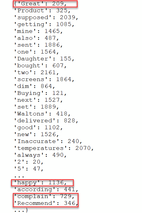
bow_transformer.vocabulary_
The vocabulary is the entire list of unique words found in the preprocessed text by the number of occurences. It is easy to see (but not always true) what words might accompany a higher ranking vs a low ranking. Some examples are highlighted in red. Also, this is a single token (single word) count. We are not looking at a n-gram (n word sequence) to evaluate the sentiment. For instance, we notice the word below, “happy”, it is currently taken in isolation. The sentiment can easily point in the negative direction and lower the ranking we are trying to derive, if “happy”is preceded by the word “not”. So that is definitely an improvement that can be made using a bi-gram or n-gram tokenization.
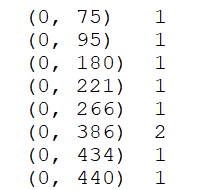
bow8 = bow_transformer.transform([reviewer8])
print(bow8)
This produces forty tokens from the original comment found in reviewer8 record. Some examples are shown below.
#check  the English word for the feature in below vectors

print (bow_transformer.get_feature_names_out()[386]) #Temp
print (bow_transformer.get_feature_names_out()[1153]) #heater
Now that we have generated the vocabulary, we need to establish the entire corpus of preprocessed reviews as a matrix of tokens. Naturally, we expect the number of rows in the matrix to be the same as number of reviews, and the number of columns in the matrix to be the same as the length of vocabulary. This brings us to the shape 1,229 records X 2,326 words, we already established above.
This is the code to generate the matrix of count vectors.
comments_bow = bow_transformer.transform(finaldf['reviewTextStr'])
print('Shape of Sparse Matrix: ', comments_bow.shape)
print('Amount of Non-Zero occurences: ', comments_bow.nnz)
print('sparsity: %.2f%%' % (100.0 * comments_bow.nnz / (comments_bow.shape[0] * comments_bow.shape[1])))
Now that we have laid the numeric ground work much needed for computation, we still have to arrive at a metric that tells us importance of a word relative to another. That is precisely what TFIDF does. TFIDF stands for Term frequency inverse document frequency. It is the product of the two terms — Term frequency and Inverse Document Frequency. Term frequency is the ratio of number of times a word occurs in a document (in our case, the entire set of reviews used for this analysis) over the total number of words. So higher the ratio, the more important the term is. Whereas, Inverse Document Frequency is the log of the ratio of total number of documents over number of documents where the term is found. Where does the inverse word come from in IDF? It comes from the idea that this term can also be expressed as the log of the inverse of the ratio of documents where the term is found. It semantically has the same meaning as our first formal definition of IDF. Basically, it’s like saying x is also the inverse of 1/x.
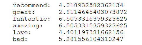
We check the TFIDF values of some words we think are important.
tfidf_transformer = TfidfTransformer().fit(comments_bow)

print(tfidf_transformer.idf_[bow_transformer.vocabulary_['recommend']])
print(tfidf_transformer.idf_[bow_transformer.vocabulary_['great']])
print(tfidf_transformer.idf_[bow_transformer.vocabulary_['fantastic']])
print(tfidf_transformer.idf_[bow_transformer.vocabulary_['amazing']])
print(tfidf_transformer.idf_[bow_transformer.vocabulary_['love']])
print(tfidf_transformer.idf_[bow_transformer.vocabulary_['bad']])
comments_tfidf = tfidf_transformer.transform(comments_bow)
Recall, our goal was to take all the text ratings and see if we can classify them into a high or low ranking. So, for that we check the distribution of our derived rating from the newrating field.
newaxisvals = finaldf['newrating'].value_counts()
plt.figure(figsize=(30, 10))
plt.subplot(131)
plt.bar(newaxisvals.index,newaxisvals.values)
plt.xticks(fontsize=18)
plt.yticks(fontsize=18)
plt.show()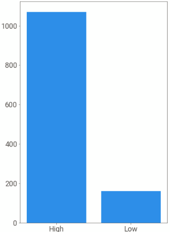
This is an unbalanced distribution, which we would have expected based on the distribution of the original ratings we saw in our initial analysis.
distratio = finaldf['newrating'].value_counts()[0] /  finaldf['newrating'].value_counts()[1]
print(distratio) # gives a value of 6.68125
The number of High ranking records is 6x times that of Low ranking. In other words, the ratio of majority class over minority class is 6x. So, before we train a classifier, we need to balance this data. Otherwise, the classifier will have a bias to incorrectly predict ratings with High ranking more than it would for Low ranking.
We apply random oversampling where the minority class is resampled so that the High and Low rankings are equally distributed. We use RandomOverSampler class to do this.
from imblearn.over_sampling import RandomOverSampler
oversampler = RandomOverSampler(sampling_strategy='minority', random_state=42)
newx, newy = oversampler.fit_resample(comments_tfidf,finaldf['newrating'])
#when you print newx you will see a sparse matrix of float64 dtype with 2138
#obsevations (upsampled from previously 1229 observations)
And a quick check shows that the data is now balanced.
newy.value_counts()
newaxisvals = newy.value_counts()
plt.figure(figsize=(30, 10))
plt.subplot(141)
plt.bar(newaxisvals.index,newaxisvals.values)
plt.xticks(fontsize=18)
plt.yticks(fontsize=18)
plt.show() 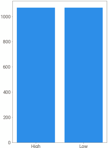
Now that we have the data ready for training the model, we partition it into test and train and then train the model, followed by checking how we fare on predicting by comparing the predicted ranking with actual ranking.
MultinomialNaiveBayesClassifier is a good model for this work as it takes a sparse matrix as an argument as X, which is exactly what we have setup and takes an array for Y. In our case it is the sentiment (ranking).
comment_train, comment_test, rating_train, rating_test = train_test_split(newx, newy, test_size=0.3)
rating_detection = MultinomialNB().fit(comment_train, rating_train)
rating_pred = rating_detection.predict(comment_test)
print(classification_report(rating_test, rating_pred))
We see a pretty good F1 score, which is a harmonic measure of precision and recall combined together as shown in the classification report below.
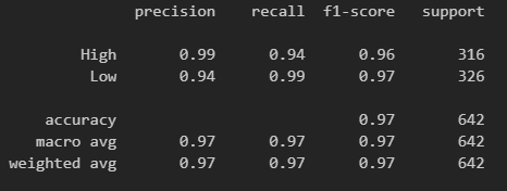
Notice both High Ranking and Low Ranking are predicted equally well.
It may be worth reiterating the significance of balancing the data. If we don’t balance the classes, the F1 score for Low Ranking suffers giving us a value of 0.5. If you are interested in seeing if this is true, you might want to run this experiment without the oversampling. Without balancing (6:1 ratio of High:Low ranking in this case), this bias skews the overall accuracy to 0.91 showing the model is highly accurate when in fact it is not.
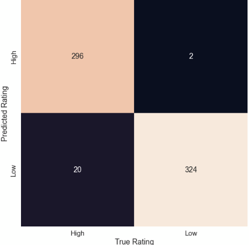
#print confusion matrix
cmat = confusion_matrix(rating_test, rating_pred)
plt.figure(figsize=(10,10))
sns.set(font_scale=1.5)
sns.heatmap(cmat.T, square=True, annot=True, fmt='d', cbar=False,
            xticklabels=['High','Low'], yticklabels=['High','Low'])

plt.xlabel('True Rating')
plt.ylabel('Predicted Rating')
The confusion matrix below shows the true positives, true negatives, false positives and false negatives.
Limitations & Improvements
There are many improvements that can be done with this experiment. We used word count as the vector for the text representation. This experiment was done for a specific type of niche product among the millions of products sold on Amazon. This specific method of vectorizing using bag of word (BOW) technique introduces sparsity exponentially as more vocabulary is introduced. Which means if there were a lot more reviews, or we open this analysis to a broader array of products, we’d run into computational issues due to the sparsity. BOW also does not take into account word order and meaning of the word. While this is a simpler technique, it has been extensively used in the past for document and text classification.
There are better ways to handle text classification. Word embeddings offer a denser representation than what we saw. It is therefore computationally efficient. By combining word embeddings with neural networks different bodies of text such as documents (or in our case reviews) can be classified.
Lastly, I’d be remiss to say that Transformers is yet another and newer way to handle text classification. I’ll cover these in future articles in natural language processing using transformer architectures.
Until next time!
References: